python, 전처리, 통계, 가설검정, 기계학습, 회귀, 분류, 군집, 모델 학습, 모델 평가
분류 모델(Classification Models)은 입력 변수(X)를 기반으로 범주형 타겟 변수(y)를 예측하는 지도 학습 모델이다. 회귀와 달리 출력이 이산적인 클래스이며, 새로운 데이터가 어느 범주에 속하는지 판단한다. 이 장에서는 로지스틱 회귀, k-NN, 결정 트리, 랜덤 포레스트 등 주요 분류 모델의 원리와 실무 활용법을 학습한다.
예제: 데이터 로드
import seaborn as snsimport pandas as pdimport numpy as npimport matplotlib.pyplot as pltfrom sklearn.model_selection import train_test_splitfrom sklearn.preprocessing import StandardScalerfrom sklearn.metrics import accuracy_score, classification_report, confusion_matrix# 데이터 로드df = sns.load_dataset("penguins").dropna()# 특성과 타겟 준비X = df[["bill_length_mm", "bill_depth_mm", "flipper_length_mm", "body_mass_g"]]y = df["species"]print("데이터 크기:", df.shape)print("\n특성 변수:", X.columns.tolist())print("타겟 변수: species (범주형)")print("\n클래스 분포:")print(y.value_counts())print(f"\n클래스 개수: {y.nunique()}")
데이터 크기: (333, 7)

특성 변수: ['bill_length_mm', 'bill_depth_mm', 'flipper_length_mm', 'body_mass_g']
타겟 변수: species (범주형)

클래스 분포:
species
Adelie       146
Gentoo       119
Chinstrap     68
Name: count, dtype: int64

클래스 개수: 3
23.1 분류의 개념
분류는 입력 데이터를 사전에 정의된 범주 중 하나로 할당하는 문제이다.
회귀 vs 분류 비교
구분
회귀 (Regression)
분류 (Classification)
출력 타입
연속형 (수치)
범주형 (클래스)
예측값
실수 값
클래스 라벨 또는 확률
예시
체중, 가격, 온도
종, 합격/불합격, 질병 유무
평가 지표
MSE, MAE, R²
정확도, 정밀도, 재현율, F1
대표 모델
선형 회귀, Ridge, Lasso
로지스틱 회귀, SVM, 결정 트리
분류 문제의 유형
유형
설명
예시
이진 분류
2개 클래스
합격/불합격, 스팸/정상
다중 클래스 분류
3개 이상 클래스
펭귄 종(3개), 손글씨 숫자(10개)
다중 레이블 분류
여러 클래스 동시 예측
영화 장르(액션+코미디)
분류 문제 예시
분야
입력 변수
출력 변수 (클래스)
의료
증상, 나이, 검사 결과
질병 유무
금융
신용 점수, 소득, 채무
대출 승인/거부
마케팅
구매 이력, 방문 빈도
이탈 여부
생물학
부리 크기, 날개 길이
종(species)
23.2 데이터 준비
예제: 학습/테스트 분할
from sklearn.pipeline import Pipeline# 데이터 분할 (stratify로 클래스 비율 유지)X_train, X_test, y_train, y_test = train_test_split( X, y, test_size=0.2, random_state=42, stratify=y # 클래스 비율 유지 (분류에서 매우 중요))print("=== 데이터 분할 ===")print(f"학습 데이터: {X_train.shape}")print(f"테스트 데이터: {X_test.shape}")# 클래스 비율 확인print("\n=== 클래스 비율 비교 ===")print("전체 데이터:")print((y.value_counts() /len(y) *100).round(1))print("\n학습 데이터:")print((y_train.value_counts() /len(y_train) *100).round(1))print("\n테스트 데이터:")print((y_test.value_counts() /len(y_test) *100).round(1))
=== 데이터 분할 ===
학습 데이터: (266, 4)
테스트 데이터: (67, 4)

=== 클래스 비율 비교 ===
전체 데이터:
species
Adelie       43.8
Gentoo       35.7
Chinstrap    20.4
Name: count, dtype: float64

학습 데이터:
species
Adelie       44.0
Gentoo       35.7
Chinstrap    20.3
Name: count, dtype: float64

테스트 데이터:
species
Adelie       43.3
Gentoo       35.8
Chinstrap    20.9
Name: count, dtype: float64
Stratify의 중요성
클래스 불균형 데이터에서 필수
학습/테스트셋의 클래스 비율 유지
편향된 평가 방지
23.3 선형 분류 모델: 로지스틱 회귀
로지스틱 회귀(Logistic Regression)는 이름은 회귀지만 분류 모델로, 선형 결정 경계를 사용한다.
# 확률 출력 (처음 5개 샘플)print("\n=== 예측 확률 (처음 5개) ===")proba_df = pd.DataFrame( y_proba_lr[:5], columns=pipe_lr.classes_)proba_df['Predicted'] = y_pred_lr[:5]proba_df['Actual'] = y_test.iloc[:5].valuesprint(proba_df.round(3))
from sklearn.tree import plot_tree# 트리 구조 시각화plt.figure(figsize=(20, 10))plot_tree(tree, feature_names=X.columns, class_names=tree.classes_, filled=True, rounded=True, fontsize=10)plt.title("Decision Tree Structure")plt.tight_layout()plt.show()
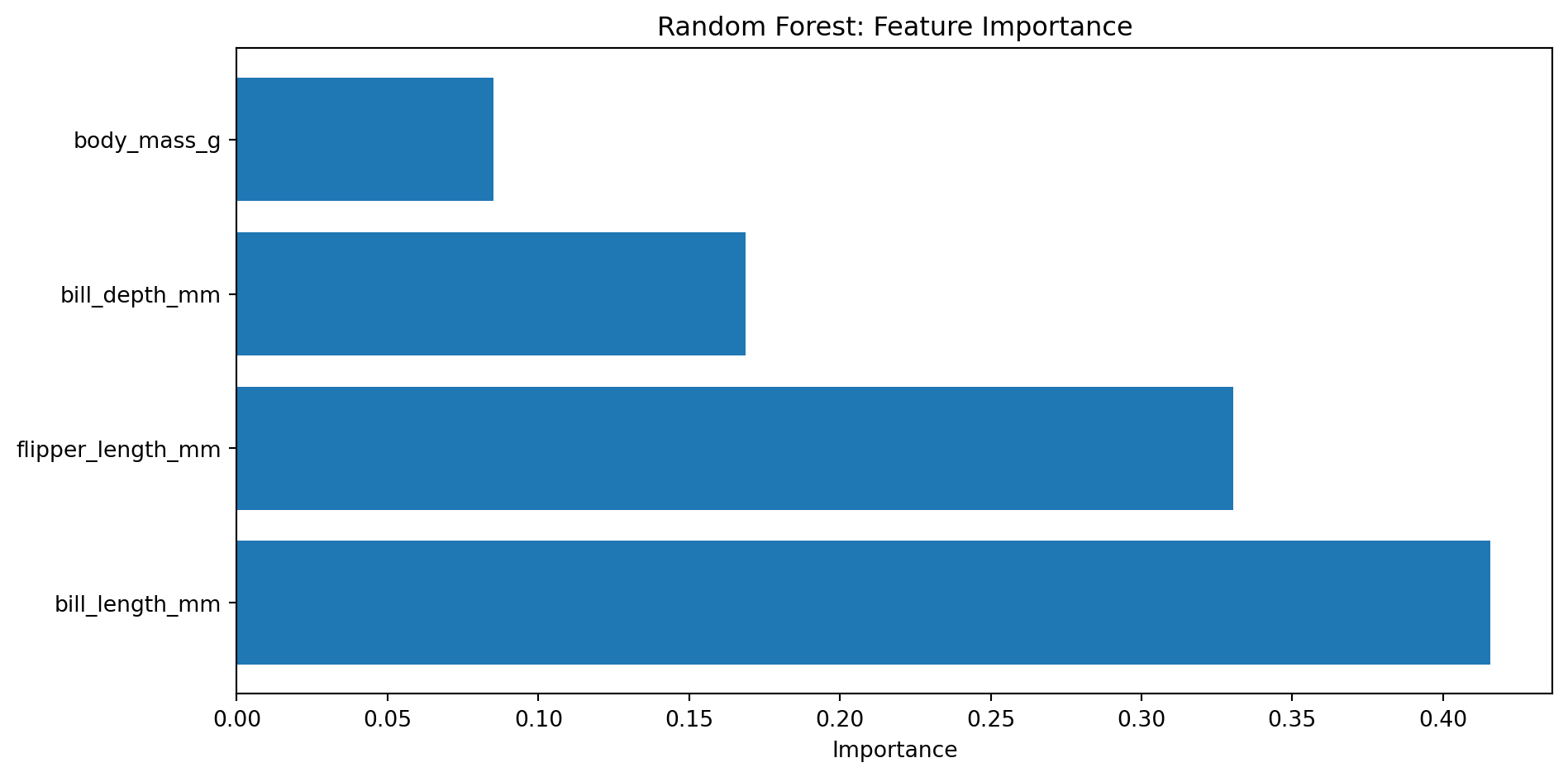
예제: 변수 중요도
# 변수 중요도importance_df = pd.DataFrame({'Feature': X.columns,'Importance': tree.feature_importances_}).sort_values('Importance', ascending=False)print("\n=== 변수 중요도 ===")print(importance_df)# 시각화plt.figure(figsize=(10, 5))plt.barh(importance_df['Feature'], importance_df['Importance'])plt.xlabel('Importance')plt.title('Decision Tree: Feature Importance')plt.tight_layout()plt.show()
# n_estimators 영향 확인n_trees = [10, 50, 100, 200, 500]accuracies_rf = []for n in n_trees: rf_temp = RandomForestClassifier(n_estimators=n, random_state=42, n_jobs=-1) rf_temp.fit(X_train, y_train) acc = rf_temp.score(X_test, y_test) accuracies_rf.append(acc)# 시각화plt.figure(figsize=(10, 6))plt.plot(n_trees, accuracies_rf, marker='o', linewidth=2)plt.xlabel('Number of Trees')plt.ylabel('Accuracy')plt.title('Random Forest: Effect of n_estimators')plt.grid(True, alpha=0.3)plt.tight_layout()plt.show()
23.7 모델 종합 비교
분류 모델 특성 비교
모델
선형성
스케일 민감
해석력
학습 속도
예측 속도
과적합
적용 상황
로지스틱 회귀
선형
높음
높음
빠름
빠름
낮음
기준 모델, 해석 중요
k-NN
비선형
매우 높음
중간
빠름
느림
중간
소규모 데이터
결정 트리
비선형
낮음
높음
빠름
빠름
높음
탐색, 설명
랜덤 포레스트
비선형
낮음
중간
느림
중간
낮음
실무, 성능 우선
예제: 모든 모델 성능 비교
# 모든 모델 성능 비교models = {'Logistic Regression': pipe_lr,'k-NN (k=5)': pipe_knn,'Decision Tree': tree,'Random Forest': rf}results = []for name, model in models.items():if name =='Logistic Regression'or name =='k-NN (k=5)': pred = model.predict(X_test)else: pred = model.predict(X_test) acc = accuracy_score(y_test, pred) results.append({'Model': name, 'Accuracy': acc})results_df = pd.DataFrame(results).sort_values('Accuracy', ascending=False)print("=== 모델 성능 비교 ===")print(results_df)# 시각화plt.figure(figsize=(10, 6))plt.barh(results_df['Model'], results_df['Accuracy'])plt.xlabel('Accuracy')plt.title('Classification Models Comparison')plt.xlim([0.8, 1.0])plt.grid(True, alpha=0.3, axis='x')plt.tight_layout()plt.show()
=== 모델 성능 비교 ===
                 Model  Accuracy
0  Logistic Regression  1.000000
1           k-NN (k=5)  1.000000
3        Random Forest  0.970149
2        Decision Tree  0.940299
23.8 모델 선택 가이드
상황별 모델 선택
상황
권장 모델
이유
빠른 기준선 필요
로지스틱 회귀
학습 빠르고 안정적
해석 중요
로지스틱 회귀, 결정 트리
계수/규칙으로 설명 가능
비선형 관계
결정 트리, 랜덤 포레스트
복잡한 경계 표현
성능 최우선
랜덤 포레스트, Gradient Boosting
앙상블로 높은 정확도
데이터 적음
k-NN, 로지스틱 회귀
과적합 위험 낮음
고차원 데이터
로지스틱 회귀 (L1/L2)
차원 저주 완화
의사결정 흐름
해석이 필수인가?
├─ Yes → 선형 관계인가?
│         ├─ Yes → 로지스틱 회귀
│         └─ No → 결정 트리
└─ No → 성능이 최우선인가?
          ├─ Yes → 랜덤 포레스트
          └─ No → 데이터 크기는?
                   ├─ 작음 → k-NN
                   └─ 큼 → 로지스틱 회귀
23.9 실무 체크리스트
분류 모델 적용 시 확인사항
23.10 요약
이 장에서는 범주형 예측을 위한 주요 분류 모델을 학습했다. 주요 내용은 다음과 같다.
분류 모델 핵심
로지스틱 회귀: 선형, 해석 가능, 기준 모델
k-NN: 거리 기반, 직관적, 스케일 민감
결정 트리: 비선형, 해석 용이, 과적합 주의
랜덤 포레스트: 앙상블, 안정적, 실무 우수
실무 권장사항
로지스틱 회귀로 시작: 빠른 기준선 확보
랜덤 포레스트로 개선: 성능 향상
하이퍼파라미터 튜닝: GridSearchCV 활용
앙상블 결합: 여러 모델 결합 고려
분류 모델은 실무에서 가장 흔한 머신러닝 문제이다. 데이터 특성과 목적에 맞는 모델을 선택하고, 적절한 전처리와 평가를 통해 최적의 성능을 달성하는 것이 중요하다.